Giving a voice to the whole population

This blog discusses different ways that population subgroups can be analysed and how sample sizes and statistical power are maintained.

Cohort studies are frequently used in the health and social sciences and typically follow samples of individuals sharing a common characteristic, such as the year that they were born, for years or even decades.

As cohort studies progress, an increasing proportion of the original sample will no longer participate, for example due to death, refusal or not being traced. In long-running cohort studies, it is natural to wonder both whether the studies remain representative of their original target populations and whether specific subgroups of people will continue to be included in the sample in sufficient numbers to allow meaningful statistical analysis – we refer to this as coverage of the subgroup.

Are the CLS cohorts nationally representative?

Here are CLS, we are home to several longstanding national longitudinal studies of people born around the same year, who have been followed since birth or adolescence. These are each nationally representative samples, drawn from the populations of England, Great Britain, or the UK.

Over time, as is inevitable in longitudinal studies, their samples have reduced and some types of people have dropped out more than others. Even when people from particular groups are less likely to participate over time, we can use simple statistical methods to ensure that analyses using the cohorts remain nationally representative, and CLS researchers have developed user-friendly guidance on how to do so.

Do the CLS cohorts have sufficient coverage of population subgroups?

Population subgroups of interest to researchers include people with protected characteristics as defined by the Equality Act 2010, such as sex, age, disability, and race. They may also include other groups defined by vulnerability, socio-demographics, health or geography. It is important to study these subgroups so that government policy can be designed for all sections of society, for example when addressing issues such as mental ill health and healthy ageing.

A lack of coverage for a given population subgroup may result in numbers so small that analysis is not possible at all or a statistically under-powered analysis from which definitive conclusions cannot be drawn. Thankfully for researchers, the CLS cohort studies retain sufficient coverage to allow meaningful analysis of many population subgroups of interest – and will likely continue to do so into the future, even as more cohort members leave the study as they age.

Showing how different population subgroups can be studied

Typical analyses that researchers may wish to undertake include those:

1. Where the population subgroup is one category of an exposure variable. We provide an example below where we want to test whether mental health differs between those who experienced childhood poverty and those who did not.
2. Where the population subgroup is of sole interest. Below we give an example of testing whether mental health differs by gender within the population subgroup defined by experiencing childhood poverty.
3. Where there is interest in whether an association or causal effect differs between one population subgroup and another. We provide an example below where we test whether the association between an exposure of interest and mental health differs between those who experienced childhood poverty and those who did not.

We shall illustrate these different types of analyses using achieved samples from the 1958 National Child Development Study (NCDS), which is based at CLS. NCDS is an ongoing study following the lives of an initial 17,415 people born in England, Scotland and Wales in a single week of 1958. In the most recent data collections in NCDS, we obtained samples of 9,137 respondents (at age 55) and 8,365 respondents (at age 62) (note the Age 62 Sweep ran for an extended period between 2020 and 2024 and the new data will be deposited at the UK Data Service in early 2025).

Comparing between population subgroups (analysis type 1)

Researchers may be interested in using NCDS data to compare the prevalence of an outcome (for example, poor mental health) between different population subgroups, one of which is small relative to the total sample (10%) and one of which is large (90%) (for example, experiencing childhood poverty (here considered as being in the poorest tenth of income) vs. not ).

For purposes of illustrating what sample sizes are sufficient to generate well-powered analyses, we have created a hypothetical example in which 30% of those who experienced childhood poverty reported poor mental health compared to 20% of those who did not experience childhood poverty. In this instance, those who experienced childhood poverty are therefore at 1.5 times greater risk of having poor mental health compared to those who did not.

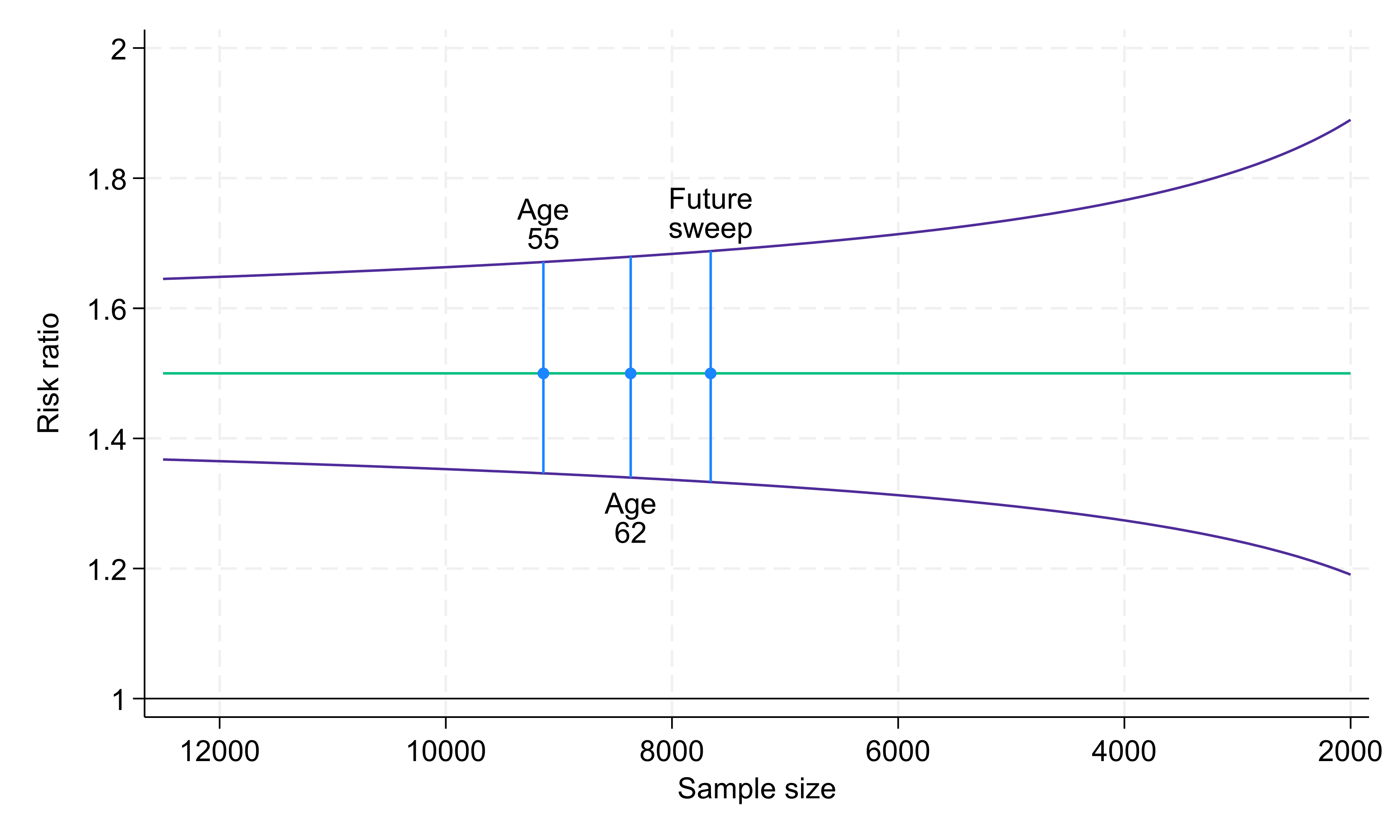
In Fig. 1 below, we apply this example to the actual sample sizes that we have achieved in NCDS in its most recent data collection sweeps, at age 55 (9,137 respondents) and at age 62 (8,365 respondents), and to a range of sample sizes that we might see in future sweeps as participants age. For the 9,137 respondents at NCDS age 55, the 95% confidence interval for this risk ratio would be (1.35, 1.67 ). This sample size results in a 95% confidence interval that lies well away from the null value of one, indicating that this analysis would provide strong evidence that the true risk ratio differed from one.

Fig. 1. Risk ratio (green line) and 95% confidence intervals (purple lines) comparing exposure groups of size 10% and 90% with 30% and 20% outcome prevalence, respectively. Sample sizes: 9,137 at age 55, 8,365 at age 62, 7,658 at future sweep (based on drop-out rate of 8.5% per sweep).

If the same exposure distribution (10% and 90%) and the same outcome prevalences (30% and 20%, respectively) were present at the current age 62 sweep, which includes 8,365 respondents, the precision with which we would estimate the risk ratio would be essentially unchanged (95% confidence interval 1.34, 1.68).

Indeed, if we project that there will be similar between-wave proportional reductions in sample sizes going forwards into the next study sweep (7,658 projected respondents), the precision would still hardly change (95% confidence interval 1.33, 1.69). Only at much smaller sample sizes would the confidence interval width increase noticeably, though even at a sample size of 2,000 (less than a quarter of the sample size achieved at age 62) the confidence interval would still be some way from the null.

It should be noted that the specific results presented here are dependent on the exposure distribution and outcome prevalences that we have assumed. For a more common minority subgroup, or a higher prevalence outcome, the confidence intervals would be narrower, whereas with an even rarer minority subgroup, or a lower prevalence outcome, the confidence intervals would be wider.

Analyses within a population subgroup (analysis type 2)

We now turn our attention to an example of an analysis conducted entirely within a population subgroup, i.e. where the population subgroup is of sole interest to the researcher, rather than in comparison with another subgroup.

Here the sample size for our analysis is not the full sample from the study sweep, but the sample we have achieved for that population subgroup. We consider a population subgroup making up 10% of the total sample (for example, those who experienced childhood poverty), within which the analysis is conducted.

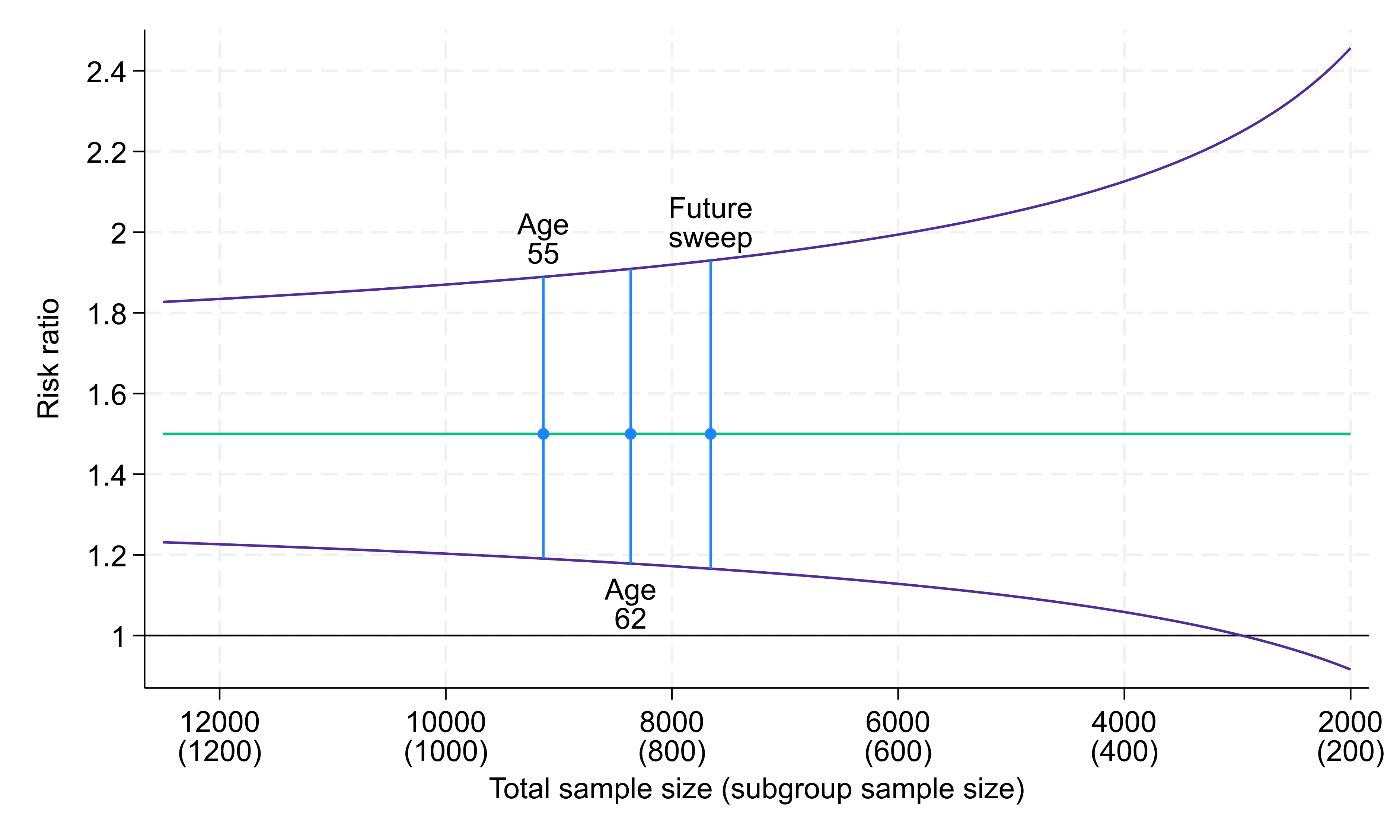
Within this 10% population subgroup we consider the risk of experiencing poor mental health between two evenly sized groups (males and females). We assume that 30% of females have poor mental health compared to 20% of males, meaning females are at 1.5 times greater risk. The age 55 NCDS sample (9,137 respondents) would give us a subgroup of 914 people within which to conduct the analysis, resulting in a 95% confidence interval for the risk ratio of (1.19, 1.89) (Fig. 2). Despite the small subgroup being analysed, this 95% confidence interval again lies somewhat away from the null value of one, providing evidence that the true risk ratio differs from one.

Fig. 2. Risk ratio (green line) and 95% confidence intervals (purple lines) for analyses within a 10% subgroup, comparing two exposure groups each of size 50%, with 30% and 20% outcome prevalence, respectively. Total sample sizes: 9,137 at age 55, 8,365 at age 62, 7,658 at future sweep.

Confidence interval width differs little at somewhat smaller total sample sizes, though for markedly smaller total sample sizes confidence intervals become wider. For example, at a total sample of around 3,000 (i.e. a subgroup analysis sample size of 300) the 95% confidence interval crosses the null, though this would constitute less than a third of the achieved sample at age 55.

Similarly to the first example, for a more common minority subgroup or a higher prevalence outcome, the confidence intervals would be narrower, whereas for an even rarer minority subgroup, for an imbalanced exposure distribution, or for a lower prevalence outcome, the confidence intervals would be wider.

Comparing associations between population subgroups (analysis type 3)

Researchers may also be interested in investigating how an association between an outcome and exposure varies between different subgroups. As an example, we might look at how the association between an exposure of interest and poor mental health differs between those who experienced childhood poverty and those who did not; in other words, is there an interaction effect? This type of analysis generally requires greater sample sizes.

As before, we assume that 10% of individuals experienced childhood poverty (and 90% did not). We now assume a binary exposure variable, distributed evenly (50% exposed and 50% unexposed) in both those who experienced childhood poverty and those who did not. We also assume that 10% of unexposed individuals had mental health issues, regardless of whether they experienced childhood poverty or not, but 20% of exposed individuals not experiencing childhood poverty and 30% of exposed individuals who did experience childhood poverty did have mental health issues – risk ratios of 2 and 3, respectively, giving a relative risk ratio of 1.5 (= 3/2). This is what we are interested in estimating here.

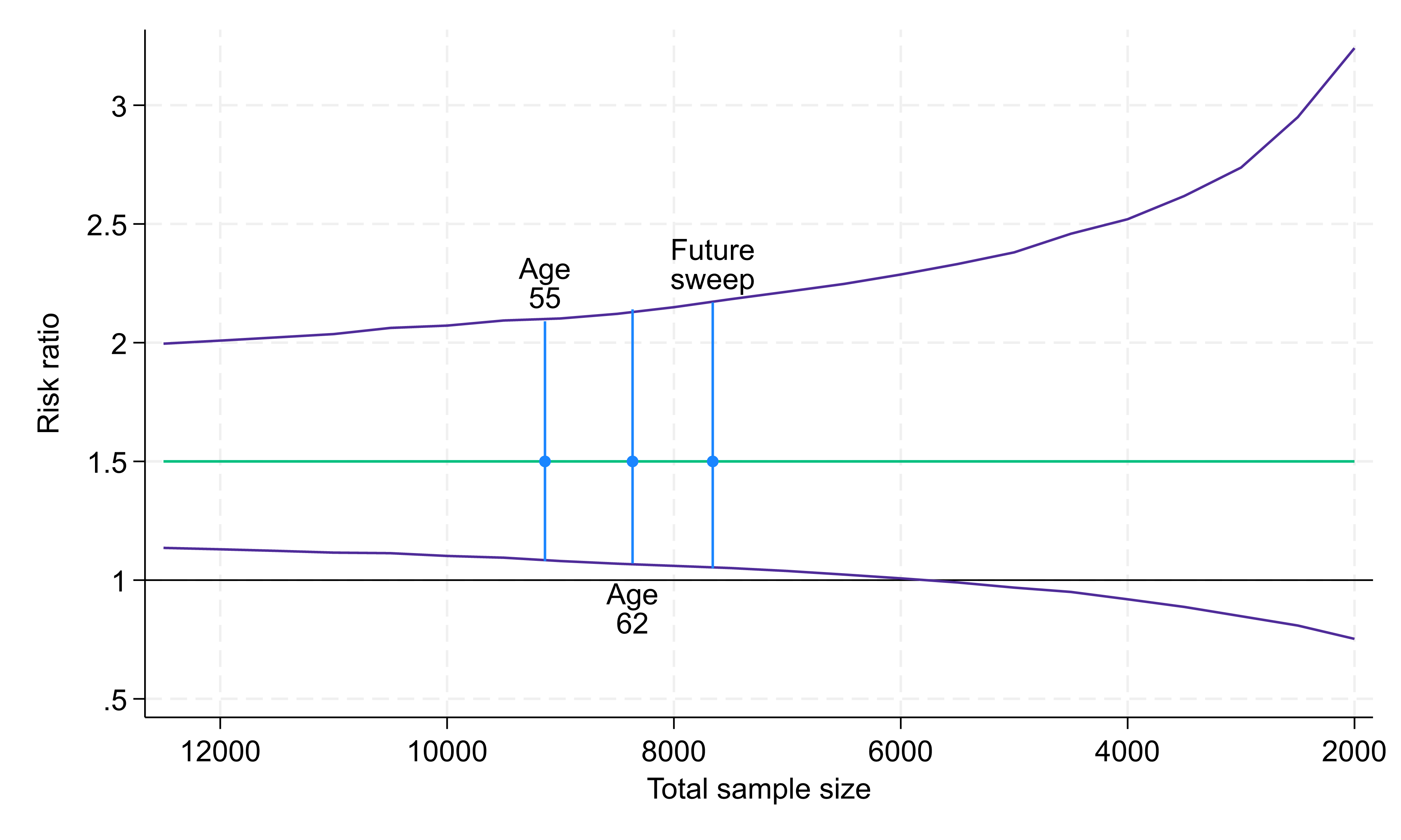
We again consider this analysis across a range of potential sample sizes (Fig. 3). At the age 55 sample size (9,137 participants) the 95% confidence interval for this risk ratio would be (1.08, 2.08). This does not (quite) include the null value of 1, providing some evidence that there is a difference in associations between the two subgroups. However, this 95% confidence interval is relatively wider than those for other example analyses, demonstrating the greater sample size typically required for this type of analysis.

For the age 62 sample size (8,365 participants) the 95% confidence interval would be (1.07, 2.14) and at a future sweep (7,658 participants) it would be (1.05, 2.17). For sample sizes below around 6,000 the 95% confidence interval would cross the null value of 1.

Fig. 3. Risk ratio (green line) and 95% confidence intervals (purple lines) for analyses comparing associations between a 10% subgroup and a 90% subgroup. Within each subgroup there are two exposure groups each of size 50%. Within the smaller subgroup the outcome prevalences are 30% and 10% in the two exposure groups (giving a risk ratio of 3) and within the larger subgroup the outcome prevalences are 20% and 10% in the two exposure groups (giving a risk ratio of 2). Total sample sizes: 9,137 at age 55, 8,365 at age 62, 7,658 at future sweep.

This is only one specific example of this type of analysis. The ability to draw conclusions about differences between associations in population subgroups will be determined by the relative sizes of the subgroups, how many people within each subgroup have experienced the exposure, and how many have experienced the outcome.

Further considerations

Study members failing to answer certain questions may mean that the sample available for specific analyses is smaller than the total number of respondents. However, by using methods such as multiple imputation we can use other information collected from study members to make up for these missing data. These study members can then be included in the analysis, increasing both statistical power and the representativeness of the analysis. The presence of particularly rich previously observed information is an important strength of these long-running national cohort studies.

The longitudinal nature of the CLS cohort studies can also be used to increase effective sample sizes (e.g., by utilising repeat measurement of outcomes or defining a characteristic as present in any of several sweeps). Further, data from across cohorts may be pooled as similar constructs have been measured in each.

Analyses of very small population subgroups

The above analyses are typical of those conducted using NCDS data and demonstrate how analyses of data from the CLS cohort studies remain well powered at current and likely future levels of response. Population subgroups of very small sizes may, however, lack sufficient coverage in the CLS cohorts.

For example, if we are interested in a rare health condition which effects only 1 in 100 people, we would expect to observe just 90 cases in a sample of 9,000 study members, making the numbers too low to draw any telling conclusions. However, these are not the scenarios that such population-representative cohort studies are designed to address; other study designs would be more fruitfully employed here.

Maintaining statistical power as the studies age

In conclusion, despite attrition over their decades-long lifespans, the CLS cohorts remain representative of their target populations when analysed appropriately. They retain sufficient coverage to allow meaningful analysis of many population subgroups of interest and will continue to do so in the future, even with further drop out.

The older CLS cohorts offer an unparalleled opportunity for the study of ageing from a life course perspective, and data collections will remain valuable even when sample sizes decline due to mortality. There are no other prospective life course studies in the world that have continued from birth through to death that have sample sizes comparable to those in the CLS cohorts, making these a precious asset as they approach their later decades.

• By Richard J. Silverwood, Liam Wright, Alissa Goodman, George B. Ploubidis, Centre for Longitudinal Studies